Catherine Hood Consulting

Diagnostics FAQ

1. What are the features of a quality seasonal adjustment?
2. What diagnostics are available in X-13ARIMA-SEATS to help us judge the quality of the adjustment?
3. What do I do if the diagnostics fail?
4. How do I "fix" failing M diagnostics?
5. How much data do I need to get diagnostics information from X-13ARIMA-SEATS?

---

1. What are the features of a quality seasonal adjustment?

The following are some of the features of a quality seasonal adjustment.

• There should not be any estimable seasonal effects in the seasonally adjusted series. The presence of seasonal and calendar effects in either the seasonally adjusted series or irregular component is referred to as residual seasonality.
• The level of the series should lack bias. A lack of bias in the level means that the local level of the series is similar for both the original and the seasonality adjusted series.

Other features are desirable, though not mutually exclusive. Many people (and also many government agencies, in my experience) prefer adjustments that are stable, meaning that as new data are added and incorporated into the estimation procedure, the revisions to the past estimates are small. Big revisions can indicate that the initial estimates are misleading or even meaningless.

Another useful feature may be smoothness, particularly if you are looking for turning points in the series. Unfortunately, a smoother series often has larger revisions.

Back to the Top

2. What diagnostics are available in X-13ARIMA-SEATS to help us judge the quality of the adjustment?

One of X-12-ARIMA's main advantages over other seasonal adjustment programs was the diagnostics, and these same diagnostics are in X-13ARIMA-SEATS

Some important diagnostics are:

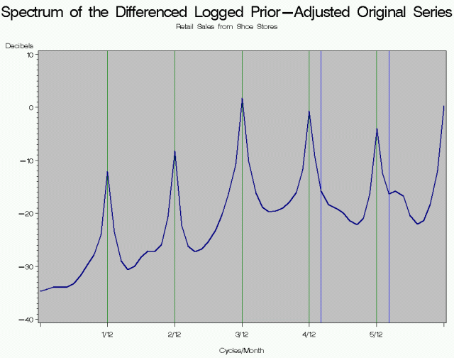
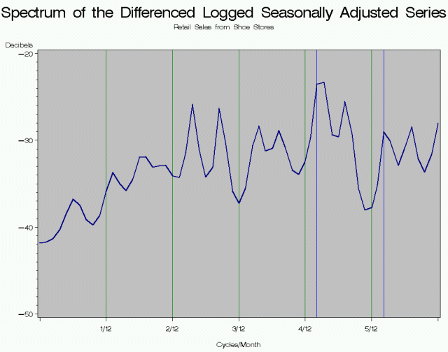
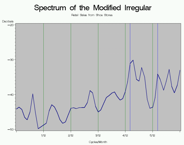
Spectral Graphs: A prominent spectrum peak at any of the seasonal frequencies for the spectrum usually indicates the presence of seasonal effects. X-12/X-13 can estimate four spectra: the spectrum of the differenced original series, the spectrum of the differenced seasonally adjusted series, the spectrum of the modified final irregular component, and the spectrum of the regARIMA model residuals.

The program warns of visually significant peaks at seasonal frequencies for monthly series of k/12 cycles/month where 1 ≤ k ≤ 5 and trading day frequencies of 0.348 and 0.432 cycles/month. For quarterly series the seasonal peaks are at 1/4 and 1/2.

We use spectral graphs of the original series to see if the series is seasonal. (If the series isn't seasonal, then there is no need to seasonally adjust the series.)

We use the spectral graphs of the irregular and the seasonally adjusted series to determine whether there is residual seasonality or residual calendar effects. We use the spectral graph of the regARIMA model residuals to see if there may be some problem with the regARIMA model.

Let's look at an example. Below is the spectrum of the original series for Retail Sales of Shoe Stores. The seasonal frequencies are marked in green and the trading day frequencies in blue. Note that the original series shows signs of very strong seasonality with peaks at the seasonal frequencies 1/12, 2/12, 3/12, 4/12, and 5/12 cycles per month.

The Graphs below show the spectrum of the seasonally adjusted series and the irregular. Notice that peaks at the seasonal frequencies are suppressed completely. This means there is no estimable seasonal effect still present in the seasonally adjusted series or in the irregular. There is a slight peak at the second trading day frequency, but because the 0.348 frequency has been suppressed, we can also conclude there is no estimable trading day effect still present in the seasonally adjusted series or in the irregular.

The problem with the spectral graphs in the output file of X-12/X-13 is that the horizontal axis is not labeled. For monthly series, the first column of S's on the left is at 1/12, the second column of S's is at 2/12, the next column is 3/12, the next at 4/12, and the next at 5/12. The far right edge of the graph is at 6/12 cycles per month. For quarterly series, the column of S's in the center is at 1/4 and the far right edge of the graph is at 2/4.

Sliding Spans: Sliding spans detect instability in the seasonally adjusted series. Sliding spans compare different estimates from the seasonal adjustment from overlapping subspans of the time series data. Some of the available estimates:

• the seasonal factors,
• the seasonally adjusted series, and
• the month-to-month (or quarter-to-quarter) change in the seasonally adjusted series.

An adjustment is considered acceptable if

• the percentage of unstable seasonal factors is less then 15%,
• the percentage of unstable seasonal adjustment values is less than 15%, and
• the percentage of unstable month-to-month (quarter-to-quarter) changes is less then 35%.

Revision Histories: Revision histories give information about stability in the seasonally adjusted series or the trend.

In history analysis, X-12/X-13 performs a sequence of modeling and/or seasonal adjustment runs on a sequence of increasing data spans, adding one point at a time to the end of the series. Available options in history spec include:

• revisions for seasonal adjustment, seasonal factors, and trend,
• month-to-month (or quarter-to-quarter) revisions for seasonal adjustment and trend,
• revisions from projected factors to final factors, and
• out-of-sample forecast errors and AICs for the regARIMA model.

M and Q Diagnostics: M and Q diagnostics were developed at Statistic Canada for X-11-ARIMA and are also included in X-12-ARIMA and X-13ARIMA-SEATS. They indicate the properties of the adjustment that are often associated with adjustments of good quality. There are 11 M statistics (M1-M11) and two Q statistics (Q and Q2). Q is the weighted average of the M statistics.

The values of Ms and Qs range from 0.0 to 3.0. Any M greater than 1.0 indicates a source of potential problems for the adjustment procedure. Keep in mind that some M diagnostics are more important than others, and not every M has to be less than one for the adjustment to be acceptable.

Among all M statistics, M7 is the most important statistic. M7 can show if there is too much moving seasonality relative to the stable seasonality. Because of the moving average procedures in X-11-ARIMA and the subsequent X-12-ARIMAa and X-13ARIMA-SEATS, too much moving seasonality may cause problems in the estimation of the series components.

There is more information on the M diagnostics in question 4 below.

More details on X-12-ARIMA seasonal adjustment diagnostics can be found in the paper "Getting Started with X-12-ARIMA Diagnostics."

Back to the Top

3. What do I do if the diagnostics fail?

The first thing to keep in mind is that for most series, not all of the diagnostics will pass, so it is not unusual to have some diagnostics failures. The best thing to do is to decide what is important for your series and rely mostly on those diagnostics.

For example, I personally believe that the most important quality of a seasonally adjusted series is that there should be no seasonality. So I rely on the spectral diagnostics the most, and then I watch the history diagnostics to check on the stability of the adjustment.

If you aren't sure what a change in the diagnostics means for your series, a course on the diagnostics can be very helpful.

Back to the Top

4. How do I "fix" failing M diagnostics?

We will discuss the individual diagnostics, separately or in groups, followed by a brief discussion of what can be done, if anything, when the diagnostic fails. Recall that any value less than 1.0 is acceptable for any M diagnostic.

M1 and M2 are designed to measure the relative strength of the variation in the irregular component versus the variation of the seasonal component. The idea is that if there is too much irregular, then the program won’t be able to separate the irregular and seasonal well. M1 and M2 test this property by using two different functions to detrend the series.

M1 is the relative contribution of the irregular over three months span. You can improve the M1 diagnostic, sometimes, with changes to the seasonal filters or to the sigma limits. I have also found that shortening the series can improve this diagnostic.

M2 is the relative contribution of the irregular component to the "stationary portion of the variance." M2 values can be misleading if the trend shows several changes of direction or in some other way is not well-approximated by a straight line. For this reason, X-12/X-13 computes Q2, a weighted average of the M statistics that excludes M2. I generally ignore failing M2 statistics.

M3 and M5 are designed to to see if there is too much irregular in the series relative to the trend. Again, the idea is that if there is too much irregular in the series, the program will not be able to separate the trend from the irregular. M3 is the amount of month-to-month change in the irregular component as compared to the amount of month-to-month change in the trend-cycle. M5 is the number of months it takes the change in the trend-cycle to surpass the amount of change in the irregular, using a statistic called "months to cyclical dominance."

Both M3 and M5 may fail if we have a series with a very flat trend because the change in the irregular will always be more than the change in the trend. For a series like this, there is nothing we can do to improve the diagnostics, but nothing needs to be done. If the series has a flat trend, X-12/X-13 can estimate it quite easily, and there is no cause for concern if M3 and/or M5 fail.

M4 tests for randomness in the irregular component using a statistic called the average duration of run. Because the irregular is not really white noise anyway, this statistic is not very important in the overall picture. It is the M statistics with the smallest weight in the Q and Q2 statistics.

In my experience, this diagnsotic will often be the only M diagnostic that passes for very bad series, and often is the only failing M diagnostic for very well-behaved series. I generally ignore failing M2 statistics.

M6 checks if a 3x5 seasonal filter is the correct seasonal filter based on the moving seasonality ratio. If the seasonal filter used in the run is not a 3x5, the program will not use M6 to compute the overall Q statistic.

If this diagnostic fails, and you are using a 3x5 filter, then you should change the seasonal filter length. If you are NOT using a 3x5 filter, or if X-12/X-13 doesn't choose a 3x5 filter for the last seasonal estimation, then you can ignore the M6 diagnostic.

M7 is the most important M statistic, and forms what X-11-ARIMA calls the "test for identifiable seasonality." It tests the amount of moving seasonality present relative to the amount of stable seasonality. Because of the moving average procedures in X-11/X-12/X-13, too much moving seasonality may cause problems in the estimation of the series components.

If this diagnostic fails, then there is probably nothing that can be done to correct it. And if it fails, then the series probably is not seasonal and should not be seasonally adjusted. There are cases when we have a short series and a very bad model, and fixing the model may fix the M7 diagnostic. Also, there are times when we have a very long series, and shortening the series can fix the M7 if the problems with the series were at the beginning of the series.

M8, M9, M10, and M11 attempt to find problems in the seasonal component. M8 uses a measure of the fluctuations in the seasonal component to see if there are too many random fluctuations in the seasonal component, which can be a sign of problems in estimating the seasonal component. M9 examines the linear movement in the seasonal component, and tries to see if the seasonal component is changing too quickly. Again, a high value can indicate problems in estimating the seasonal factors. M10 and M11 are the same statistics as M8 and m9, but they are calculated for only the last few years of the series. M10 and M11 give us insight into the quality of the most recent estimates of the seasonal factors.

High values for M8 and M9 may be fixed with changes to the seasonal filters or to the sigma limits, or again, by shortening the series if the series has changed or there are problems at the beginning of the series. High values of M10 and M11 are difficult to fix, and the only solution is to keep watch on the series for signs of other problems down the road.

Back to the Top

5. How much data do I need to get diagnostics information from X-12-ARIMA and X-13ARIMA-SEATS?

You need five years of monthly data and 15 years of quarterly data (60 data points) to get fairly good spectral estimates.

To be able to use the revision diagnostics, you may need as few as seven years, but as many as 12 years of data. For series with 3x9 filters, it may be useful to have 15 years of data for the revision history and sliding spans diagnostics. Most series will probably use a 3x5 filter which uses seven years of data, so you will need about 10 years to get revision diagnostics and useful sliding spans information.

Back to the Top

Continue with the next set of questions on Trouble-Shooting